Confidence intervals

Confidence intervals (CIs) provide an estimation of a true value within a population, and some type of certainty around that value. The certainty that is constructed can be a little confusion, and perhaps misleading. It is often communicated with less-than-desirable terminology and phrasing.

Objectives

1. Provide basic formula for computing a CI for a sample
2. Provide an accurate definition of the CI
3. Demonstrate the concept of the CI with visual aids

Parameters

\[ \begin{array}{l,l,c,r} \text{sample n} & n &=& 100 \\ \text{population mean} & \mu &=& 5 \\ \text{population standard deviation} & \sigma &=& 2 \\ \text{alpha level} & \alpha &=& 0.95 \end{array} \]

Code

set.seed(20220804)
n <- 100
mu <- 5
sigma <- 2
alpha <- 0.95

do_sample <- function() {
  # n, mu, sigma defined outside
  rnorm(n, mu, sigma) 
}

x <- do_sample()
s <- sd(x)
xbar <- mean(x)
z <- qnorm((1 - alpha) / 2, lower.tail = FALSE)

Name	Value
Mean \(\bar{x}\)	5.4082339
Standard deviation \(s\)	1.9219276
Z-score (\(z\))	1.959964

Confidence interval (objective 1, objective 2)

\[ \text{CI}_\mathit{mean}\ =\ \bar{x}\ \pm\ Z_{\alpha/2}\ \times \mathit{se} \\ \]

When we construct a confidence interval, we are doing so with our specific sample of the population. We are using the mean of the sample as well as the standard deviation.

The certainty in the confidence interval is not directly but indirectly linked back to the true population. When we construct a .95 CI, we are constructing a range of values from a sample, and in doing so are making the assertion that were we to construct CIs for other samples within this population, that approximately 95% of those confidence intervals would contain the true population parameter. The .95 certainty is not the certainty that the true population parameter is within our given confidence interval. ¹

¹ This is so common that we have to have a section in Wikipedia about this: Confidence intervals: Common misconceptions. This phrase is likely how I’ve been taught and is present within the textbook from my own graduate classes.

Sampling demonstration

If we want to check this assumption, we can get 100 new samples and compute the confidence intervals for each of those.

Code

do_mean_ci <- function(xbar, s) {
  # n, z defined outside
  se <- s / sqrt(n)
  se_z <- se * z
  c(lower = xbar - se_z, upper = xbar + se_z)
}

sem <- do_mean_ci(xbar, s)

r_mean_ci <- replicate(100, {
  r_x <- do_sample()
  r_xbar <- mean(r_x)
  r_sd <- sd(r_x)
  do_mean_ci(r_xbar, r_sd)
})

str(r_mean_ci)
#>  num [1:2, 1:100] 4.77 5.55 4.76 5.52 4.63 ...
#>  - attr(*, "dimnames")=List of 2
#>   ..$ : chr [1:2] "lower" "upper"
#>   ..$ : NULL

Just for the plotting, we’re going to sort of the r_mean_ci matrix by the mean value of upper and lower. This doesn’t effect our analysis.

Code

# reorder by mean of ranges -- simply for visuals
r_mean_ci <- r_mean_ci[, order(apply(r_mean_ci, 2L, mean))]

Now we can check against this array of intervals, how many contain our population mean, .

Code

are_between <- r_mean_ci["lower", ] < mu & r_mean_ci["upper", ] > mu
mean(are_between)
#> [1] 0.96

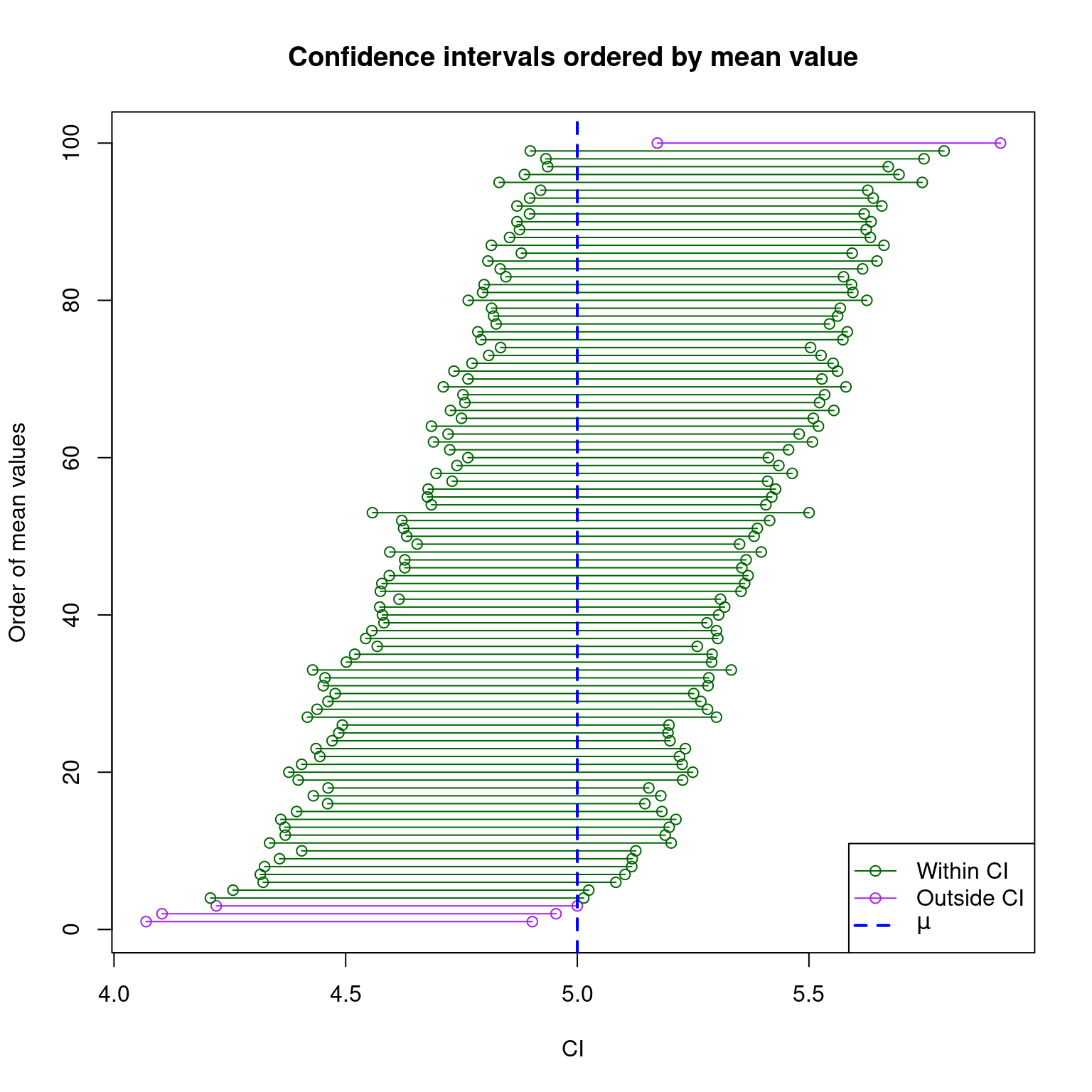
Plotting confidence intervals (objective 3)

We’re seeing that sum(are_between) of our 100 replications do contain the true population mean, . These are estimations, so we’re always going to get exactly 95 of 100.

We can also plot these confidence intervals.

Code

# plot the points
plot(
  x = c(r_mean_ci["lower", ], r_mean_ci["upper", ]),
  y = c(1:100, 1:100),
  col = ifelse(c(are_between, are_between), "darkgreen", "purple"),
  main = "Confidence intervals ordered by mean value",
  xlab = "CI",
  ylab = "Order of mean values"
)

# connect points with lines
segments(
  r_mean_ci["lower", ], 
  1:100, 
  r_mean_ci["upper", ], 
  1:100,
  col = ifelse(are_between, "darkgreen", "purple") ,
)

# add vertical line for mu
abline(v = mu, col = "blue", lwd = 2, lty = 2)

# provide legend
legend(
  "bottomright",
  c("Within CI", "Outside CI", expression(mu)),
  col = c("darkgreen", "purple", "blue"),
  lty = c(1, 1, 2),
  lwd = c(1, 1, 2),
  pch = c(1, 1, NA)
)